
Workload Forecasting: Give Leadership a Range, Not a Single Date15 min read

A steering committee asks a fair question. When will the six projects we committed to this year land?
The portfolio lead does the responsible thing:
- Break the work down into tasks
- Estimate each piece with the people who will do it
- Roll the numbers up into a schedule
- Put a single date on a slide
Then the date slips anyway, even with careful estimates and a team that hit every number it promised.
The estimate forecast the project and ignored the system it runs inside. Two variables set the real date, and neither one survives a roll-up.
Leadership needs a range, a confidence level as soon as the record can carry one, and a method that earns both.
Why Bottom-Up Estimates Break in Innovation Portfolios
Estimate-and-roll-up is a reasonable method. It just carries assumptions that innovation work quietly violates:
- The work is well enough understood to decompose accurately
- Assigned capacity is genuinely dedicated
- Sequence stays stable once planning ends
- A delay on one project doesn’t touch the others
Break any one of those and the arithmetic still produces a date. It just stops meaning anything.
The cone of uncertainty describes the honest version. At the earliest stage of a project, estimates properly carry a band of roughly four times in both directions.
That cone narrows as work proceeds, but only if scope holds still. In innovation portfolios scope moves, and a moving scope re-widens the cone.
Where the Estimation Bias Actually Comes From
The classic planning fallacy research put hard numbers on the gap:
- Honours students predicted their theses would take 33.9 days
- The work actually took 55.5 days
- Only 29.7% finished by their own predicted date
- In a separate study within the same paper, 74% of participants’ reported thoughts ran forward into the plan, and only 7% looked backward at how similar work had actually gone
Experience doesn’t inoculate anyone against this, because the mechanism is directional. Bent Flyvbjerg’s project database shows the same pattern at scale.
Nine out of ten megaprojects overrun on cost, and overruns up to 50% in real terms are common.
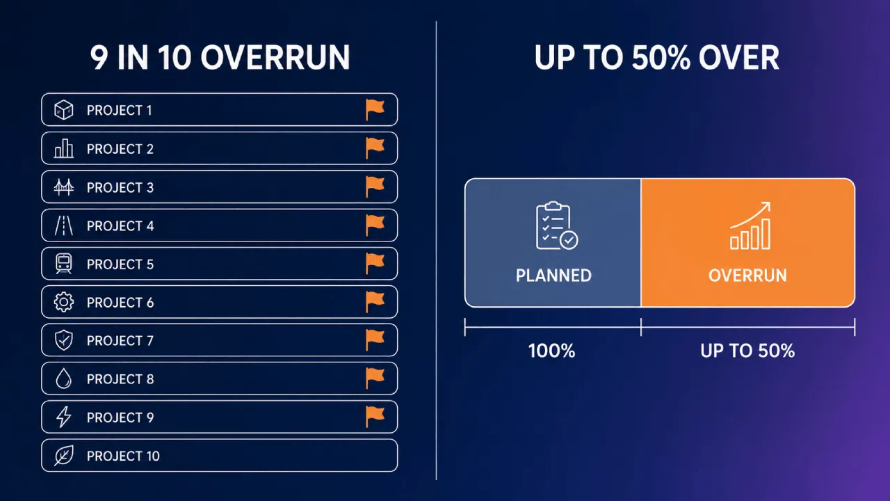
That’s the cost record at billion-dollar scale. An innovation portfolio running on fractional capacity has no reason to expect better on schedule.
One note on evidence hygiene, since this topic attracts sloppy citation. The widely repeated claim that roughly one in three projects succeeds traces back to an unpublished methodology.
Academic researchers have challenged it directly, surveying 193 experienced IT project managers and finding more than 90% of projects scored above mid-level success. Forecast from evidence you can inspect.
The Two Variables That Actually Set Your Delivery Date
Both of these sit outside the project plan, which is why estimating harder never fixes them. Start with the one nobody models.
Utilization, and Why 90% Busy Is Not 90% Productive
Queueing theory has an uncomfortable result for anyone who plans capacity in a spreadsheet.
Kingman’s formula expresses average wait time as a function of three things: utilization, variability, and service time. The utilization term is the one that bites.
The table below is an illustrative wait-time proxy, and the shape is what matters more than the exact multiples.
| Team Utilization | Relative Wait Time | What It Feels Like In Practice |
|---|---|---|
| 50% | 1x | Work starts when it arrives |
| 80% | ~4x | The tipping point; responsiveness degrades |
| 90% | ~9x | Everything is in progress, nothing finishes |
| 99% | ~99x | The queue governs the date, not the work |
Wait time scales with the ratio of utilization to remaining capacity, so it quadruples between half load and 80%, then runs away as you approach full load.
Don Reinertsen’s benchmark contrast sharpens the practical point. Manufacturing organisations typically cap utilization around 85%, while engineering work, he notes, often gets loaded to 95%.

That second figure sits well past the point where the curve turns steep. And innovation portfolios rarely have even that much room to play with.
Many of them run on people with day jobs. A “20% allocation” is a fractional claim on someone already sitting at or near full utilization somewhere else.
So it rarely buys 20% of a free calendar. Spreadsheets add percentages; queues add wait time.
Work in Progress, the Lever You Can Actually Pull
Little’s Law states the relationship plainly: average cycle time equals average work in progress divided by average throughput. Three variables, one equation, no room to negotiate.
Throughput is hard to raise quickly. Hiring takes months, and skilled capacity in innovation work is rarely fungible.
So the only lever that moves cycle time in the near term is work in progress. Reduce what’s in flight and things finish sooner, without anyone working faster.
The cost of ignoring that lever shows up in how fragmented the work becomes. Gloria Mark’s 2005 field study of information workers put three numbers on it:
- Roughly 11 minutes on a working sphere before switching to something else
- 57% of work segments interrupted
- An average of 2.26 intervening working spheres before interrupted work resumed the same day
That study measures individual attention rather than portfolio load. Still, it prices the switch that a portfolio with too much in flight keeps buying.
The same Reinertsen talk adds the governance half of the problem. Ask ten stakeholders to value the same piece of work without a shared model of cost of delay.
Their cost-of-delay figures will vary by something on the order of 50 to 1. That spread is what “everything is high priority” looks like once you measure it.
That’s a forecasting defect. A portfolio with no agreed priority ordering has no stable sequence to forecast against.
Four Forecasting Methods That Survive Uncertainty
Four methods hold up when the work is genuinely uncertain. What separates them is what they demand from your data.
| Method | What It Needs From You | Best Suited To | Where It Breaks |
|---|---|---|---|
| Throughput-based | Completion history, consistent work unit, count or range of work remaining | Teams with any delivery record | Wildly heterogeneous work items |
| Monte Carlo | ~20+ historical data points, scope range | Stable, repeatable delivery flow | Thin history, false precision |
| Reference class | A defined class of comparable projects | Work new to you, with comparables elsewhere | Class defined too favourably |
| Rolling wave | A live governance cadence | Stage-gated portfolios | Scope that never settles |
None of these methods removes uncertainty. Each misleads in a specific way: when data is thin, when it’s wrongly framed, or when the work never holds still.
Pick on the basis of what you can actually evidence today. A board pack rewards the most sophisticated-looking output, and your delivery record rarely supports it.
Throughput-Based Forecasting
The empirical approach forecasts from how fast you’ve actually delivered comparable work. It skips the plan and the team’s guess about what the next item should take.
Daniel Vacanti’s rule is the discipline here: never forecast from an average. An average tells you nothing without the distribution behind it.
Put a date on an average and you have committed at a confidence level nobody has stated.
For a single item, the mechanics work like this:
- Plot the cycle times of completed items on a scatter plot
- Draw the 50th and 85th percentile lines across the plot
- Read the two durations off those lines, each with its probability attached
Throughput forecasting has the lowest barrier to entry of the four. It needs your completion history, a consistent unit of work, and a count or range of what’s left.
That unit is also the failure mode. A backlog mixing a two-day tweak with a two-month build gives a distribution of nothing in particular.

For a batch, divide the work remaining by a weekly completion rate. Run it at a median week and at a slow week to get an unlabelled bracket.
Unlabelled is the honest word. Dividing by a slow week assumes every remaining week is slow, so the far end overshoots the longer the batch runs.
Real percentiles on a batch need the simulation in the next section.
Monte Carlo Simulation
The mechanics are straightforward. Assign probability distributions to the uncertain inputs based on historical data, then run the model repeatedly with random draws.
Monte Carlo methods commonly run thousands of simulations, often 10,000 or more. The output is a curve of probabilities.
A worked example from Expedia Group’s engineering teams shows the shape of the output, if not a model data set. Their inputs were modest:
- Completed-throughput data from the past seven sprints
- A low/high range for remaining scope
- A story-splitting factor to account for scope uncertainty
Five hundred runs were enough, though seven sprints is thin by the standard set below. Stakeholders picked a date against their risk appetite: 7% early, 50% mid, 85% late.
The accuracy evidence holds where the data supports it. One peer-reviewed study put Monte Carlo delivery-date forecasts at 32% mean magnitude of relative error.
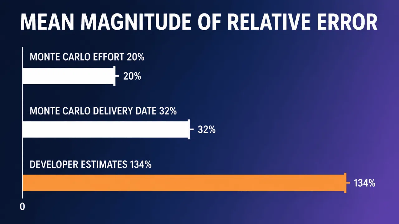
Its effort forecasts landed at 20%, against 134% for the developers’ own estimates.
The same study found accuracy stabilised once roughly 20 historical data points existed. That threshold is the honest constraint on this method.
Below it, Monte Carlo still runs, producing confident-looking output from almost no signal. That’s worse than saying you don’t know.
Reference Class Forecasting
Reference class forecasting swaps your project’s plan for the record of projects like it. Three steps:
- Build a class of genuinely comparable completed projects
- Establish the distribution of their actual outcomes
- Locate the new project inside that distribution
That’s the outside view, judging the project by its class instead of by the plan it wrote for itself. It’s deliberately impersonal, and that’s the point.
It’s the strongest option for work you’ve never done before, which describes a large share of any real innovation portfolio.
It borrows the history you don’t have from a class you can define. It also carries credibility with a sceptical steering committee.
The UK was the first European government to make the method mandatory for cost estimation on state-sponsored transport projects, and Denmark followed shortly after.
The failure mode sits entirely in class definition. A class assembled to flatter the project is an inside view wearing a costume.
Rolling Wave Re-Forecasting at Gates
“Plan a little, do a little.” In practice that means three things:
- Detailed planning for the near horizon
- Placeholder detail for the far one
- A genuine re-forecast at each gate
A PMI-published practitioner paper builds the idea into a six-step process for innovation programmes, and it maps onto how most portfolios already run.
Stage-gated portfolios get this almost for free. Each gate is already a decision point, so the change is purely procedural: make a re-forecast a required gate output.
The failure mode is subtle. Re-forecasting only narrows the cone if scope is genuinely settling between gates.
Run it on a project whose scope keeps moving and you just re-document the same uncertainty against a newer date. The ritual happens, the information doesn’t improve.
Matching the Method to Your Portfolio’s Data Maturity
Your delivery record, the novelty of the work, and your governance structure decide which method you’ve earned. Match them honestly:
- Fewer than about 20 observations of whatever you would sample, item cycle times or per-sprint throughput. Use cycle-time percentiles for single items and an unlabelled bracket for batches. Impose a WIP limit and skip simulation entirely.
- A stable record of 20 or more such observations. Monte Carlo earns its keep here, and the accuracy gap over point estimates is real.
- Work that’s new to your organisation but not to the world. Reference class forecasting, even if you have a throughput record, with throughput percentiles kept for the routine items around it. If no comparable class can be assembled, the method isn’t available to you.
- A stage-gated portfolio with a governance cadence already running. Layer rolling wave re-forecasting on top of whichever of the above fits the underlying work.
The trade-off worth being blunt about is Monte Carlo on a thin dataset. It’s precision theatre, and a simulation output tends to end the conversation.
A range with visible assumptions invites challenge instead. In a governance meeting that’s the outcome you want when the data is thin.
Most innovation portfolios should start with throughput percentiles and a WIP limit, then earn their way to simulation as the delivery record accumulates.
That sequence costs nothing. And it builds the data the fancier method will eventually need.
How to Report a Range to People Who Want a Date
The real objection to probabilistic forecasting is political. Leadership asked for a date, and a committee that gets a probability distribution instead can reasonably read that as an evasion.
Answering a governance question with a chart reads as a dodge, and sometimes it is one. The reframe that lands is risk appetite.
“50% by June, 85% by August” is leadership choosing how much schedule risk to carry. Early date, more risk; later date, more certainty.
A usable forecast statement contains four things:
- The date range itself
- The confidence level attached to each date, or a plain statement that there isn’t one
- The assumptions held constant: scope, allocation, and WIP limits
- The trigger that forces a re-forecast before the next scheduled one
That last item is what separates a forecast from a wish. Naming the trigger in advance narrows the argument about whether things have changed enough to revisit the number.
Governance also tends to conflate two things worth keeping apart:
| Forecast | Commitment | |
|---|---|---|
| What it is | What the data says | A decision to accept schedule risk at a chosen percentile |
| Where it belongs | Reporting and re-planning | A contract, with the percentile attached |
Confusing the two is how teams commit to a 50% date. The practitioner record on making the switch is encouraging.
At John Lewis & Partners, one team was spending as much as 10% of its annual capacity on estimation alone.
The team switched to Monte Carlo fed by throughput data they already had, and three things followed:
- The estimation sessions stopped entirely
- Two large fixed-date commitments were delivered on time in the same week
- Two years of follow-on data showed high accuracy for a fraction of the effort
To be fair, there’s a gap in the evidence worth naming.
No controlled study establishes that executives accept probabilistic reporting better than point dates. What exists points the right direction, short of proof.
Anyone selling you certainty on that question is overstating what’s known.
What This Requires From Your Portfolio Data
Throughput, Monte Carlo, and any rolling wave built on them share one prerequisite. You need a clean, consistent record of when work entered and left each stage.
A portfolio that can’t measure can’t forecast from its own record. The method choice is downstream of a data problem nobody has framed as one.
The minimum viable data set is short:
- Stage entry and exit timestamps for every item
- A consistent unit of work, tagged by type so you can compare like with like
- An explicit definition of done for each stage
- A named owner per item
- Remaining scope as a low-high range, for every committed item whether started or not
None of that is exotic, but it has to be captured the same way every time, by everyone. Tooling only records what discipline already produces.
Ambition has outrun operational maturity almost everywhere. A 2024 BCG study of more than 1,000 senior innovation executives found 83% rank innovation in their top three priorities.
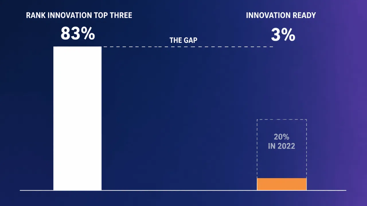
Only 3% of companies qualify as innovation-ready on BCG’s own maturity scoring, down from 20% two years earlier. The intent is there; the operational record isn’t.
Forecasting sits squarely inside that gap, and closing it is a records problem before it’s a method problem.
You can’t forecast a portfolio you can’t see, and structure in the record makes it visible.
Forecast the System, Not the Project
Most portfolios can improve their forecasts this quarter without buying anything new. What has to change is what gets reported, and how much runs at once.
Three moves, in this order:
- Put a WIP limit on the portfolio before buying any forecasting sophistication
- Replace single dates with percentiles where you have them, and state the assumptions beside them
- Make a re-forecast a required output at every gate, rather than an occasional favour
The WIP limit earns its place first because it shortens cycle time, the one lever available before you have data. Nothing else here works that fast.
None of it holds without structure in the record. Give leadership the range, and the confidence level wherever the data earns one.
Get the system predictable, and the date stops being a guess.
Download our free ebook Project Portfolio: From Opportunities to Value to learn how to structure portfolio governance and track progress and health across your initiatives.
Request a demo to see how Accept Mission gives you stage-level delivery history, real-time portfolio visibility, and reporting from one source across every innovation project.








 English
 Dutch
Dutch Portuguese
 Spanish
 French
 German
 Arabic